Object detection is bothclassifying and locating objects inside an image. In other words, it is acombination of image classification and object localisation.Building a machine learning model for image classification is simpler and Ihave described it in one of my posts here. However,an image classifier cannot tell where exactly an object is located inside an image. To achieve this we need to build a neural network which can locate anobject inside the image in addition to classifying it. In this post I am going to describe how I built a neural network for object detection by solving boththese problems.

The Object to detect

Since my intention was to build the model from scratch without spending too much time on data preparation, I picked the simplest possible object I could think of. My choice was to make a simple red color vision marker using a piece of cardboard. Since the vision marker was just a 2D shape, the different angles from which it can be captured is limited — hence the limited number of images required for the training set. I made the vision marker circular shaped and palm sized for simplicity and ease of handling.

Vision marker made usinga piece of cardboard

Architecture of the Model

Before diving into the implementation details, I thought of describing you the architecture of the model. First of all, my objective was to infer two answers:

·        Whether or not the image has the object in it

·        Where exactly is the object located

To solve the first problem, I could use an image classifier — a convolutional neural network withtwo output neurones. One of those output neurones could represent the presence of the object whereas the other one could represent the absence of it. In otherwords, the output of the image classifier is a probability distribution among the different object classes — or in this case, the presence (“Circle”)or absence (“No-Circle”) of the object. The class with the highest probability could then be determined by applying the Softmax function at the output layer.

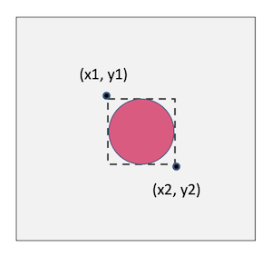
Solving the second problem was completely different. What I wanted there was to locate the object by drawing a bounding box around it. To do that, I had to find the pixel coordinates of the top left corner and the bottom right corner of the bounding box. This means my neural network had to figure out the x, y coordinates ofthose two points inside the image. I could do this by designing a convolutional neural network having 4 neurones in the output layer — representing the 4 numerical coordinate values.

Then the challenge wasto achieve these two objectives using a single neural network. On the one hand,the image classifier part of the solution treats the values of the output neurones as a probability distribution. Then it picks the one with the highest probability and takes its label as the answer. On the other hand, the object localisation part of the solution requires the 4 output neurones to give the actual bounding box coordinates. Therefore, it is difficult for the neural network to train its fully connected dense layers to fulfil both these requirements simultaneously. Because, optimising the weights and biases for the classification would jeopardise the output of the localisation, and vice versa.

The solution to this problem was to design a neural network with two branched outputs. Since the feature extraction has to be performed equally for both problems, I made the convolution layers common and sharable. However, after the convolution layers I branched the network into two — each with their own dense layers and outputl ayer to achieve the two different outcomes.

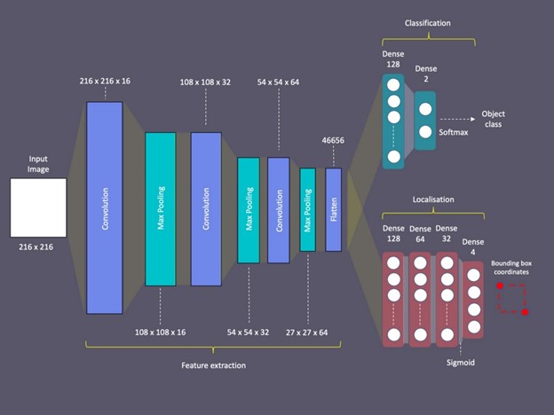
Architecture of the dual headed neural network

This architecture allowed me to train these two heads or branches with different loss functionsand activation functions. Moreover, this allowed me to train them separately using different datasets. I will describe how I did this and why it was important to do so later in this post.

Data preparation

As with any other machine learning project, data preparation was the key here too. First I configured my camera to capture square shaped images by setting the image resolution to 2160x 2160. Then I took around 126 photos of the vision marker placing it in different positions inside the image frame and placing it at varied distances to the camera. Moreover I took them with different backgrounds. These variations in the training dataset helped the model to achieve more accurate predictions at the end.

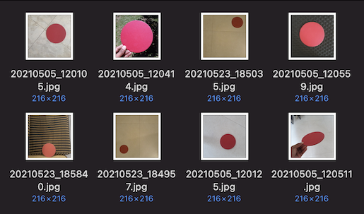
Part of the training image set

I took another 62 photos without the vision marker in them. This was done to train the model to identify the absence of the marker. Then I resized all photos to be just 216×216 pixelsin resolution as it was unnecessary to use higher resolution images for identifying such a simple object.

Image annotation

The next step was to annotate the vision markers using bounding boxes. This is an important step in building an object localiser unlike in an image classifier. I used the free and open-source annotation tool called VoTT for this purpose.

First I created a project in VoTT called “Vision marker detector”, and created the source and the target connections pointing respectively to the folder locations in my computerfor source images and the generated annotations.

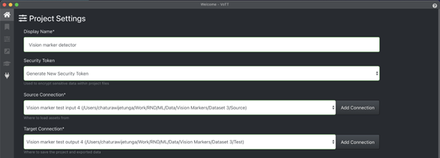
Creating a project inVoTT for the annotation task

Moreover, I created a tag (label) called “Circle” for annotating the vision markers in images.

Added a tag named“Circle”

Then it was time for the not so interesting task of annotating the images!

Example annotation inVoTT

The photos taken without the vision markers were just skipped here. I will describe how I used theseimages for the training later in this post. However, I made sure the following settingin export settings was set to generate the annotation XML files for the unassigned (non labeled) images too.

Set to export unassignedimages too

After the tedious task of annotating the images, I exported all annotations to the PASCAL VOCformat using the export option in VoTT.

Organising the folder structure

I divided the images and the corresponding annotation xml files into two sets — one to represent the training set and the other to represent the validation set.

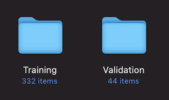
Training and validation images + annotation XML files

Then I moved them into aparent folder called “Images” inside the project folder structure.

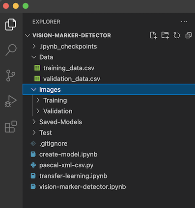
Project folder structure in VS Code

Creating the datasets

In addition to the images and their labels it is important to use the bounding box coordinates inthe process of preparing a dataset for training an object detector. For this purpose I used a python script which reads all the xml files produced by VoTT and generates two CSV files for the training and validation datasets. Ihave written this script in such a way that I could run it with the configuration variable — SKIP_NEGATIVE set to True or False to exclude or include the negative images (images without the object in them).

view raw vision-marker-detector-csv-generator.rb hosted with ❤ by GitHub

Then I wrote the following code to create the training datasets by reading the training_data.csvfile which was generated by the above step. Here I created 3 lists — first onefor the list of image data arrays, and then the second and third lists for the corresponding bounding box coordinates and the image labels respectively.

view raw vision-marker-detector-create-datasets.rb hosted with ❤ by GitHub

I used the same code toload the validation dataset as well. Then I used the following code to covert the lists to numpy arrays.

train_images =np.array(train_images)
train_targets = np.array(train_targets)
train_labels = np.array(train_labels)validation_images =np.array(validation_images)
validation_targets = np.array(validation_targets)
validation_labels = np.array(validation_labels)

When training the model,train_images array was used as the input data parameter (or parameter x)to the fit method of the Model class in Keras API.Then the arrays — train_targets and train_labels were used together in a dictionary as the target parameter (or the parameter y) to the fit method. You will notice this later in this post.

Building the model

Then it was time to build the model!

First I imported the necessary dependencies into the script.

import matplotlib.pyplotas plt
import numpy as np
import os
import PIL
import tensorflow as tffrom tensorflow import keras
from tensorflow.keras import layers
from tensorflow.keras.models import Sequential
import pathlib
import pandas as pd
from PIL import Image
from PIL.ImageDraw import Draw

I created some configuration parameters in the form of variables and defined the array of classes used for the model.

width = 216
height = 216
num_classes = 2classes = ["Circle","No-Circle"]

Then I wrote the code for defining the model. Firstly, I defined the input layer followed by are scaling layer to transform the pixel data onto the numerical value range 0–1.Then I created the convolution layers chaining the output of one layer to the input of the next. I named all these convolution layers with the prefix — “bl_”with the intention of grabbing them later using this prefix.

view raw vision-marker-detector-base-layers.rb hosted with ❤ by GitHub

Secondly, I defined the classification branch layers by inputting the flattened output from the convolution layers as per the architecture discussed before. Here I added only two dense layers — one with 128 neurones and the last one with just 2 neurones corresponding to the two class labels we have to predict. Moreover, I gave theprefix “cl_” for the layers of the classification branch.

view rawvision-marker-detector-classifier-branch.rb hosted with ❤ by GitHub

Thirdly, I defined the localisation branch layers once again inputting the flattened output from the convolution layers. Here I added 4 separate dense layers with decreasing numberof neurones ending with 4 neurones at the last layer corresponding to the 4 bounding box coordinate values used for the prediction. The layers in this branch were named with the prefix — “bb_”.

view rawvision-marker-detector-localiser-branch.rb hosted with ❤ by GitHub

Finally, it was time tocreate the model class by passing the input layer and the two output branches.This is where we weld the two output branches into the base model.

model = tf.keras.Model(input_layer,
         outputs=[classifier_branch,locator_branch])

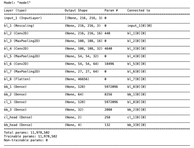
The summary of the model looked like below

Compiling the model

Since the two output branches were designed to achieve two different outcomes (one to output a probability distribution and the other to predict the actual bounding boxvalues), it was necessary to set the appropriate loss functions to each branch.I used the Sparse Categorical Cross entropy loss function for theclassification head and the Mean Squared Error (MSE) for the localiser head. I achieved this by defining the following dictionary.

view rawvision-marker-detector-losses.rb hosted with ❤ by GitHub

Then I used that together with the Adam optimisation method and compiled the model.

model.compile(loss=losses,optimizer='Adam', metrics=['accuracy'])

Training the model for localisation — bounding box regression

As I have described inthe model architecture section, my plan was to first train the model for object localisation. During this part of the training the localisation branch of themodel will perform a bounding box regression and then will adjust its weights and biases optimising for bounding box predictions.

The important thing hereis that I used only the annotated images (only the images featuring the visionmarkers) for training the localisation part of the model. I achieved this byrunning the CSV generation script with the SKIP_NEGATIVES parameter set toTrue, before running the dataset generation code as described in the dataset creation section above.

The reason for skipping the negative images (images without the vision marker) when training the localisation branch is that otherwise it affects the accuracy of the bounding box predictions. Because we have to set dummy bounding box coordinate values —such as (0,0) (0,0) for negative images if we use them too in the training dataset. For example the following chart shows how the training performance looks like for the localisation branch, if we train with both positive and negative images in the training set.

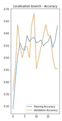
Validation accuracy is much lower when trained with negative images

However, the down side ofusing only positive image for training the localisation branch is that it gives false positives for negative images. But since I had no intention of relying onthe localisation branch to determine the presence or absence of the visionmarker, this wasn’t a problem to me.

I used the following code which defines two dictionary objects for the training and validation targets of the two named branches — cl_head and bb_head. Here you’ll notice that the labels array was for the classification branch and the bounding box coordinates array was for the localisation branch.

trainTargets = {
   "cl_head":train_labels,
   "bb_head":train_targets
}validationTargets = {
   "cl_head":validation_labels,
   "bb_head":validation_targets
}

I set the number of epochs to 20 and the batch_size to 4 initially. Then I ran the following code to train the model.

history = model.fit(train_images,trainTargets,
           validation_data=(validation_images, validationTargets),
           batch_size=4,
           epochs=training_epochs,
           shuffle=True,
           verbose=1)

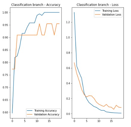
The following charts show the training performance of the two branches.

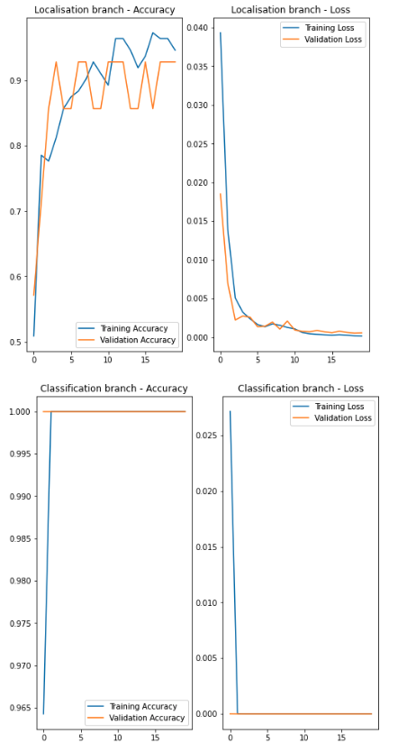
You will notice in theabove charts that the localisation branch has performed reasonably well.However, the accuracy achieved by the classification branch is too good to betrue. The performance of it was untrustworthy as it had not seen any negative images thus far. This would mean that the model (the classification part of it)will always classify what it sees as a “vision marker” since it has never seen anything without it.

However, the model wasstill capable of predicting the bounding boxes accurately even at this stage.

But then again, it gave false positives when used against negative images, giving some random bounding box coordinates as expected.

This is what I wanted tosolve by training the classification branch next.

Training the model for classification

Then it was then time totrain the classification branch of the model.

The difference here is that we need to use both positive and negative images for training the classifier as the model needs to learn both the presence and absence of images to correctly classify the images it sees.

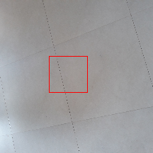
To achieve this I once again ran the CSV generation script, however by setting the SKIP_NEGATIVESparameter to False this time. This generated the CSV files containing therecords for both positive and negative images. For the negative images it created records with all zeros for the bounding box coordinates and assigned the tag — “No-Circle” as the label.

CSV file with both positive and negative images

The rest of the steps increating the new dataset were the same as creating the dataset for training the localisation branch.

The other importantthing I did before training the model in the second phase was preserving the already trained weights and biases of the convolution layers and the localisation branch. Because, otherwise a fresh round of training with adifferent set of images could have jeopardised the already trained weights andbiases of these layers resulting in declined performance. The solution for this was to freeze the convolution layers and the bounding box branch before training the classification branch with the new dataset.

I achieved this bygrabbing the base layers and the localisation branch layers using theirrespective prefixes and setting the trainable property of each layer to False.

for layer inmodel.layers:
   iflayer.name.startswith('bl_'):
       layer.trainable= False
       
for layer in model.layers:
   iflayer.name.startswith('bb_'):
       layer.trainable= False

After this step there was a significant number of Non-trainable parameters in the model. It was visible in the model’s summary.

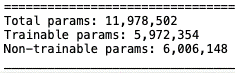
6M+ Non-trainable parameters in the model

Then I used the second dataset including both the positive and negative images to train the model.Since the base layers and the localisation branch layers were freezed, it could essentially train the localisation layers only. The training performance of the classification branch wasn’t too bad for just 20 epochs as shown in the following chart.

‍

Using the model for objectdetection

Then came the fun part of using the model to do some predictions.

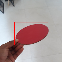
I used a new set ofphotos taken with and without the vision marker to test some predictions. Here the localiser output always gave a bounding box even if there wasn’t a visionmarker in it. But this is not a problem in an application as we can always relyon the classification output first, to know whether the object is present orabsent in the image, and then avoid drawing the bounding box if its not present. I used the same technique when displaying the below images and their bounding boxes in Jupyter notebook.

Detections by the vision marker detector

Conclusion

This exercise proved tome that we could build a simple single-class object detector from scratch without relying on large pre-trained models. Secondly, the dual headed architecture and the two phase training with different datasets was the key inachieving this result. The model gave a couple of false positives and false negatives, but this was mainly due to the limited training dataset and thenon-optimum hyper parameters. We will be able to achieve better results bytuning the hyper parameters and using a larger training dataset.

‍